The cost structure of near-real-time CDC analytics

We build ISK (Iceberg Service for Kafka), so this isn't vendor-independent analysis - but we've tried hard to make it a fair one. The cost structure below is the reason ISK exists, and it's clear enough on its own that we haven't needed to inflate anything: list prices, no negotiated discounts, every soft assumption flagged, and the incumbents' cheapest viable configuration costed honestly. 

Ballpark model for Snowflake and Databricks · list prices, US-East, no discounts · freshness ≤5 min · ranges are workload-shaped · sources at the end.

Near-real-time CDC analytics looks like it should be cheap. The data is small - a busy mid-market change feed is 50 GB/day, about 3 MB/s. You could stream that over a home broadband connection. So why do the bills land in six figures?

Cost = table-count × commit-cadence

Because the expensive thing isn't moving the bytes. It's turning a change-log into a queryable current-state table - continuous reconciliation: a dedup-by-key, paid per table, per commit, on the freshness clock. And the byte payload per commit is noise next to the fixed per-commit overhead - micro-partition or data-file rewrite, deletion vectors, a new snapshot, a metadata/log append, auto-compaction. That overhead is irreducible at a given freshness. Every approach pays it; the only question is where.

Which means the cost is driven by how many tables you keep fresh and how often each one commits - not by data volume. A 10 kB/s account table costs about the same to keep fresh as a 1 MB/s order table, because the tax is per-commit, not per-byte.

There are three ways to pay it. This model prices all three at ≤5-minute freshness.

New to the plumbing these three sit on? The pipeline appendix at the end shows where the append-only landing fits and why it forces a merge (Mode A) or a read-time union (Mode B) on top.

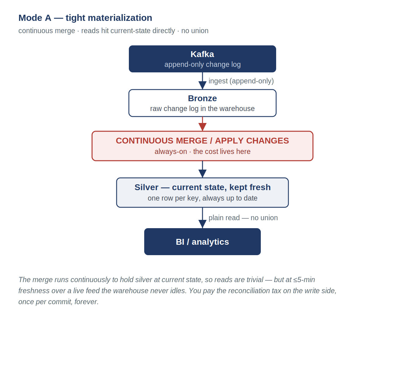
• Mode A - tight materialization. A continuous bronze→silver dedup MERGE at a tight target lag, across all tables (Snowflake Dynamic Tables / Streams+Tasks; Databricks APPLY CHANGES / Lakeflow Declarative Pipelines). At ≤5 min over a continuous feed, the staggered MERGEs of dozens of tables keep a shared warehouse effectively always-on - it pays the tax as a continuous compute bill, and write-amplification against a growing silver makes it worse over time.
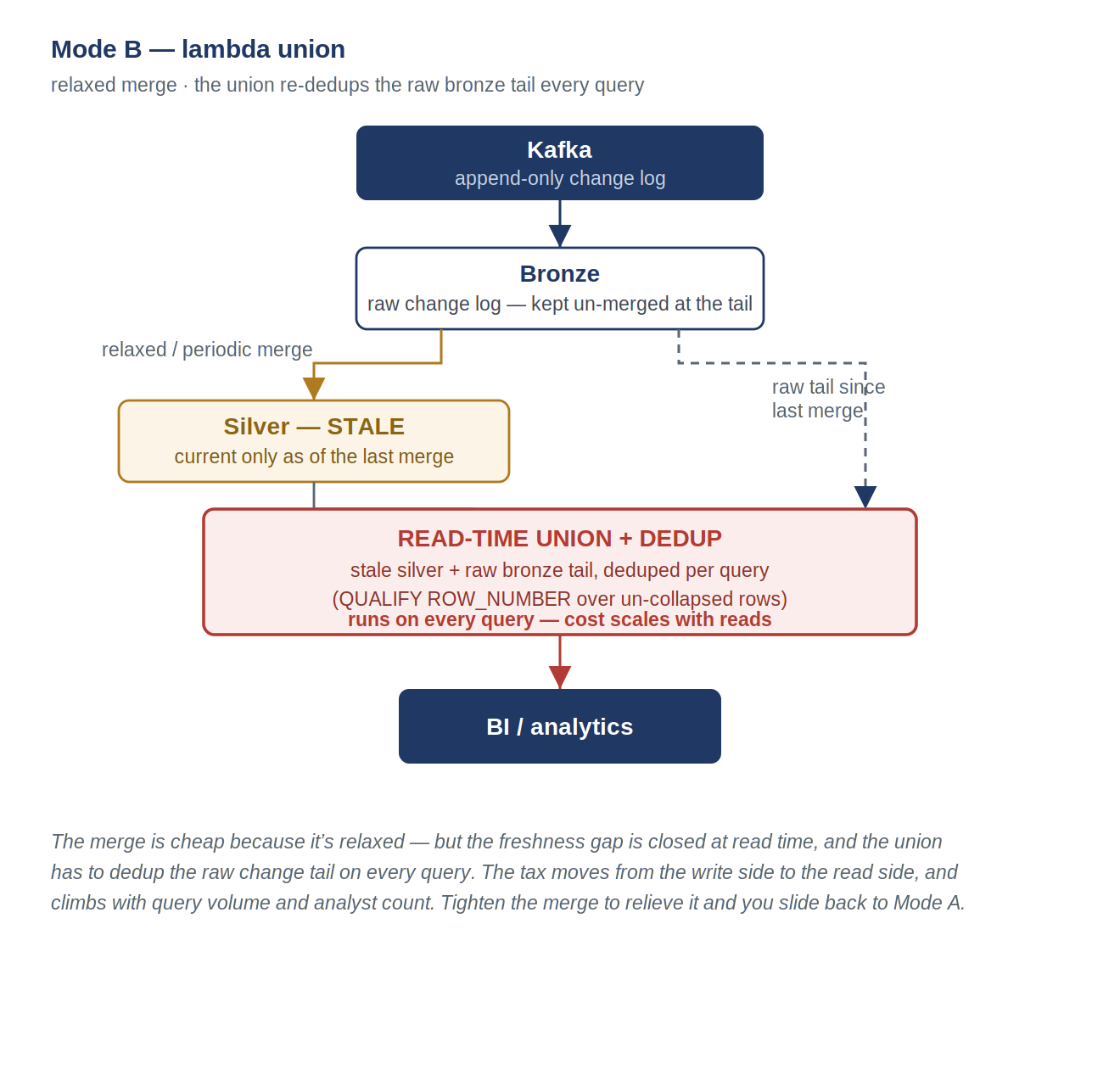
• Mode B - lambda union. Relax the merge to a cheap cadence, then close the freshness gap with a read-time dedup union over the un-merged bronze tail. It pays the tax in reads (plus, on Snowflake, billed cloud-services metadata) - and both scale with how many people query the fresh data.
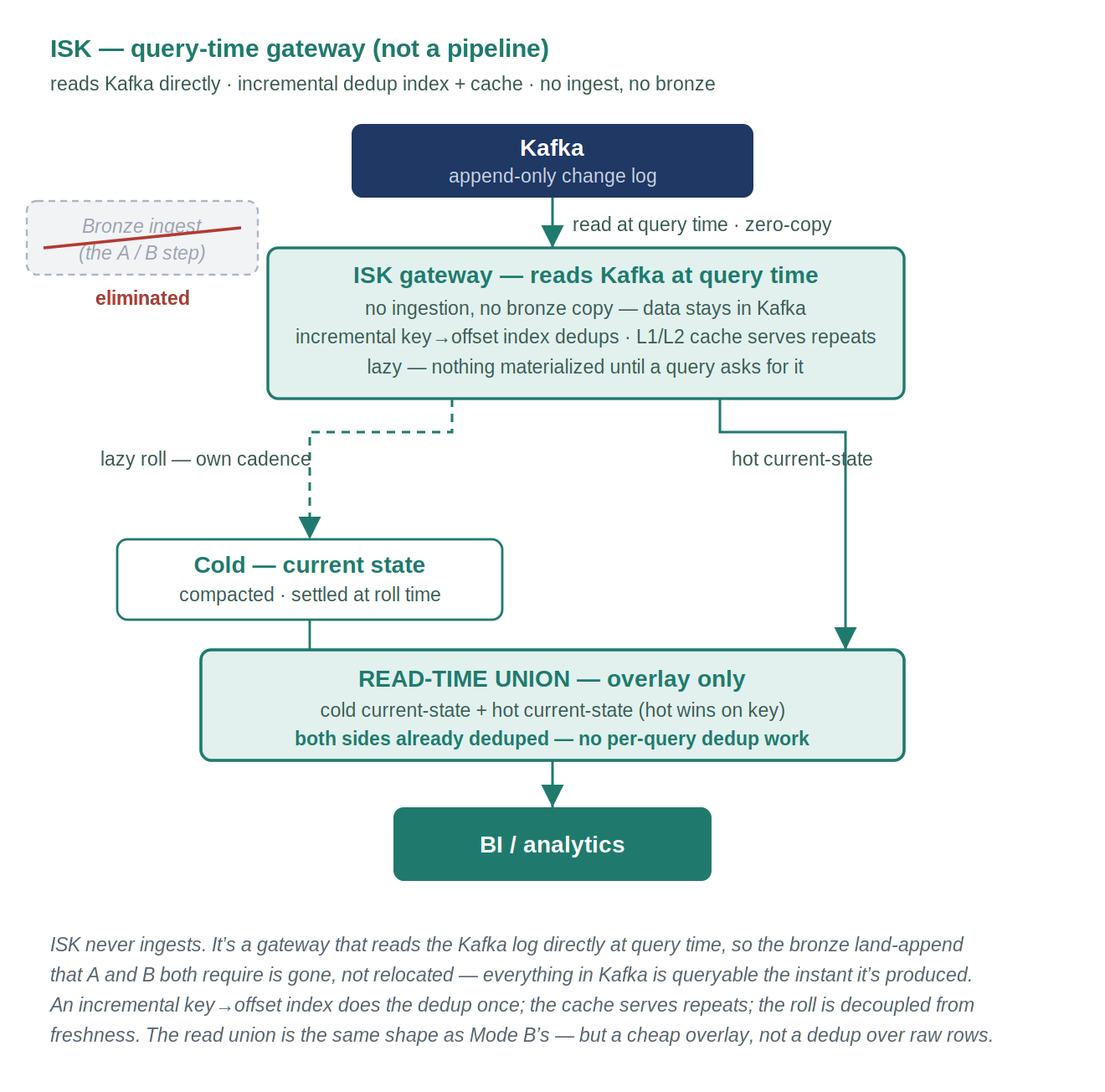
• A hot-head architecture - ISK (Iceberg Service for Kafka). Dedup is done incrementally, effectively once, off the warehouse's metered planes, on a commodity box that serves every table already-deduped from cache. Each table then rolls to the customer's compacted cold table (Iceberg, or warehouse-native) lazily, at its own volume-appropriate cadence. The dedup happens once; the freshness clock and the commit cadence are decoupled.

Cold storage and clean cold reads are held at par across all three and excluded from the comparison - analysts query a compacted current-state table either way, and that data lives in the same Snowflake / Databricks / Iceberg estate either way. The numbers below are the reconciliation cost, and nothing else.

Worked example - M, 50 GB/day 

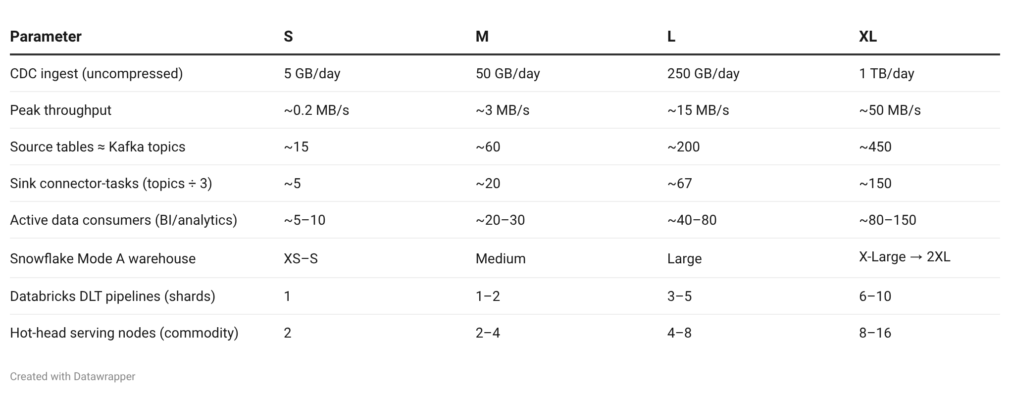
Take the middle tier on Snowflake. 50 GB/day is ~3 MB/s - trivial throughput. But it's ~60 source tables, and at ≤5-minute freshness over a continuous feed, a Dynamic Table / Streams+Tasks MERGE holding all 60 fresh runs effectively always-on warehouse: $90–105k/year, and write-amplification against a growing silver trends it upward.

Relax to a lambda (Mode B) and you trade that for a cheaper merge ($8–18k) plus a read-time dedup tax ($15–50k) plus billed cloud-services metadata ($5–18k) - ~$28–86k, with the read and metadata terms rising as more analysts query the fresh layer.

ISK's hot-head infra for the same workload is ~$5–9k (Snowflake-paired) to ~$6–11k (Databricks-paired): the same 2–4 commodity m6i.large nodes either way - two are enough at M, four is headroom for heavy query load - serving every table fresh from a local cache that, at ~4× CDC compression and a small settled hot window, fits in commodity-instance memory. Only the lazy roll to cold differs by destination (in-Snowflake, or Jobs/spot for Databricks). On Databricks the same workload's continuous APPLY CHANGES pipeline lands in the same range - $67–123k - sized not by the trivial data but by the driver coordinating 60 always-on streams (one report saturates an 8-vCPU driver at ~26 tables), with auto-compaction running inline on that cluster and periodic OPTIMIZE + deletion-vector purge stacked on top. Same work as Snowflake, same ballpark cost - against that same commodity ISK footprint.

‍

The low-volume tail is where the gap is widest

The instinct, looking at Mode A, is to triage: keep the high-churn order tables fresh, let the sleepy little dimension tables refresh slowly. It doesn't work, and the reason is worth being precise about.

Freshness is a property of the query, not the table.

Join a current order to an account dimension and the result is only as fresh as the stalest input. For any query that needs the dimension's current state, a current fact joined to an hour-stale dimension returns a silently wrong answer - the row reflects an account state that no longer exists, and nothing errors. No exception, no null, no warning. Just a quietly incorrect number on a dashboard. (A deliberate point-in-time / SCD2 "as-of" join is the exception - it's correct by construction; the trap is the far more common current-state join.)

So you can't relax a joined dimension without poisoning every real-time query that touches it. The incumbent has to hold the entire real-time join graph at the tightest cadence any consumer needs - which drags the whole low-volume dimensional tail (accounts, products, statuses: little data, many tables) up to top cadence, paying the full continuous per-table tax to deliver almost no change volume.

So the gap is widest exactly where the incumbent looks cheapest - the long tail of tiny tables. ISK serves every table fresh from the head, so a current order joins a current account with no per-table cadence decision and no staleness to propagate, while each table still rolls to cold lazily. The incumbent's only lever to cut the tail produces wrong answers.

One honest caveat for the careful reader: genuinely isolated tables - an append-only log, or a dimension used only in nightly batch with nothing real-time joining to it - can refresh slowly on either system. The hot-head approach is no worse on them, and the claim simply doesn't apply. The precise claim is about every table in the real-time join graph.

What it costs

Reconciliation cost only - cold storage and clean cold reads held at par and excluded. Ranges reflect workload shape (churn ratio, key scatter, read concurrency, silver size).

‍

‍

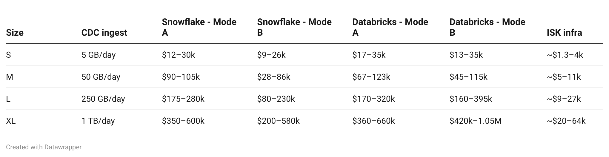
Mode A is the naive baseline most teams reach for first; Mode B is the credible, cost-conscious answer - and Why the cheap configuration doesn't stay cheap (below) explains why even Mode B doesn't stay cheap.

The shape is the same on both platforms: cost tracks the table/flow count, not the bytes (the workload is nowhere near throughput-bound - XL is ~50 MB/s). It scales roughly with the per-tier table count, not with ingest volume. That's the tell that this is a per-commit coordination tax, not a data-processing cost - and it's why the win is platform-agnostic: deletion vectors, copy-on-write, and cloud-services tiering are second-order footnotes next to the fan-out cadence tax that all commit-based table formats share.

Detail for M, both platforms:

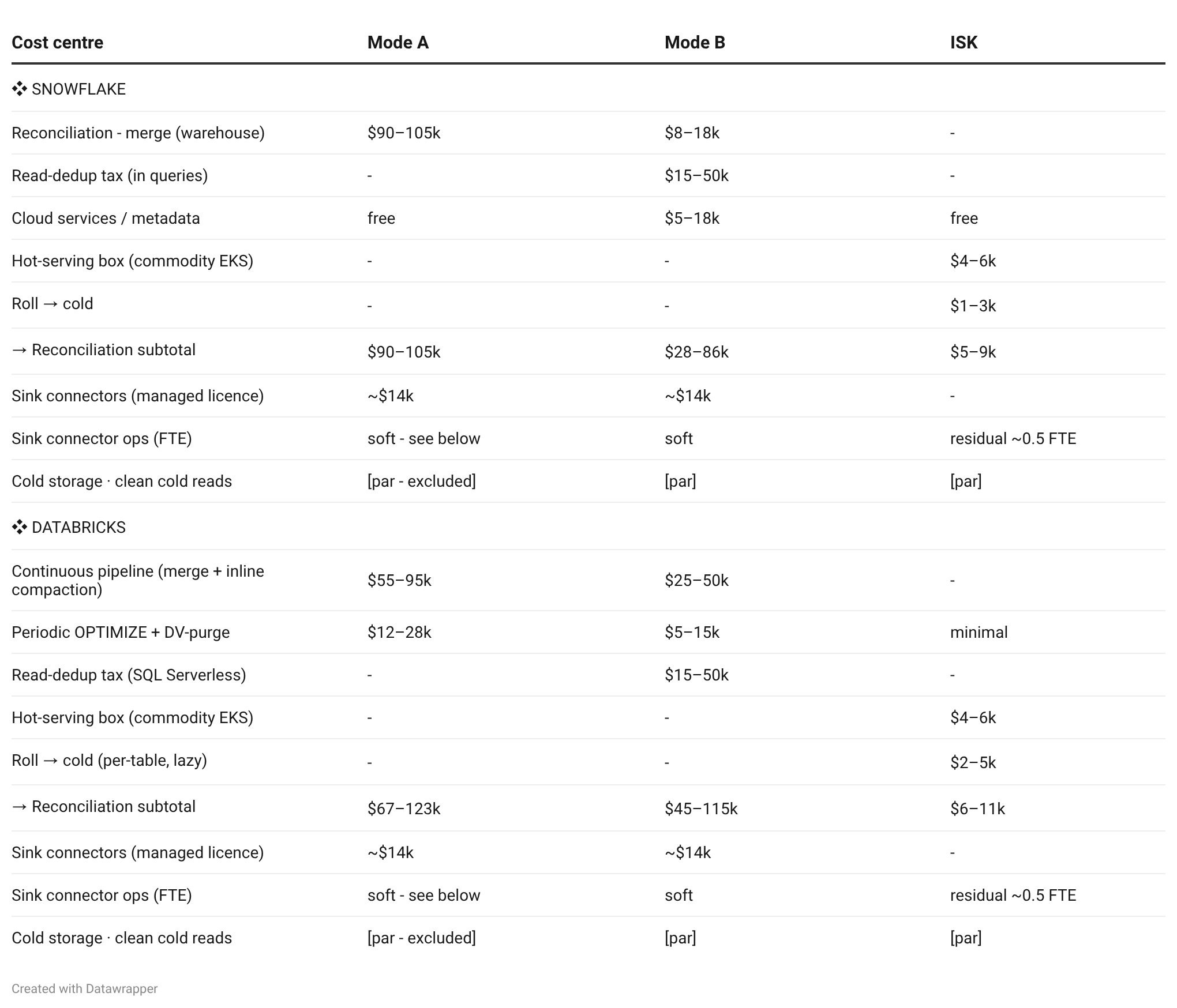
The connector lines are deliberately not summed into the reconciliation subtotal - they're a separate cost that stacks on top, and they turn out to be the bigger story. More on that below.

Other tiers (reference)

S - 5 GB/day (~15 tables)

‍

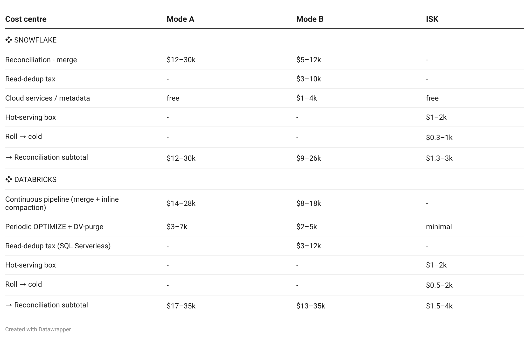
Sink connectors at S: ~$3.5k managed licence + ~0.25–0.5 FTE ops.

L - 250 GB/day (~200 tables)

‍

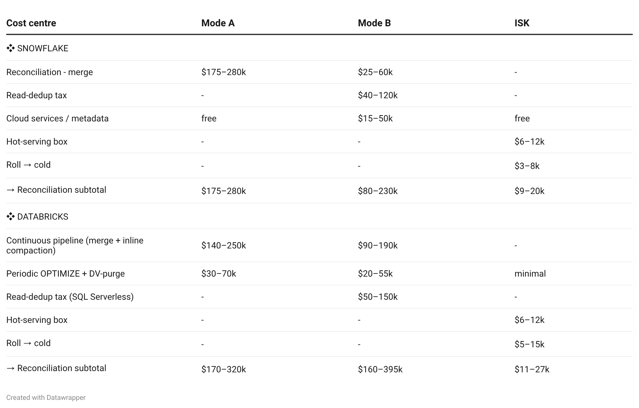
At ~200 tables the driver can't coordinate that many streams, so Databricks shards into 3–5 always-on pipelines, each its own driver - the floor multiplies, which is what holds it near Snowflake at this scale. Sink connectors at L: ~$47k managed licence + ~1.5–3 FTE ops.

XL - 1 TB/day (~450 tables)

‍

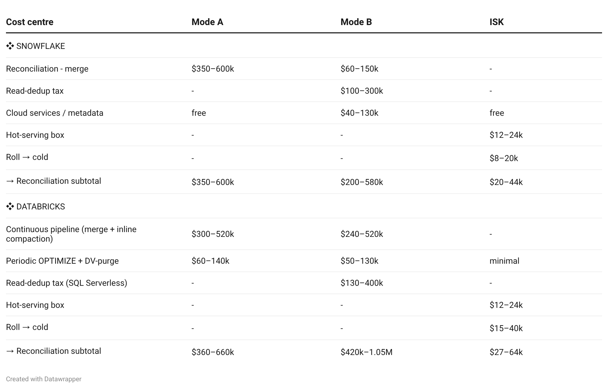
~450 streams force 6–10 always-on driver pipelines, plus heavy periodic OPTIMIZE / DV-purge under the churn - the sharding floor is what keeps Databricks tracking Snowflake at this scale. Sink connectors at XL: ~$105k managed licence + ~3–6 FTE ops.

Why the cheap configuration doesn't stay cheap

The sharp objection to all of this is "I'd run Mode B." Fair - a well-tuned lambda is the most credible incumbent answer, and at low query volume it is genuinely cheaper than Mode A. That's why teams reach for it. But it's cheaper only up to a point: Mode B doesn't have a price, it has a slope. It runs uphill along exactly the two axes a successful data product grows on - query volume and analyst count - climbing back toward Mode A's always-on cost as adoption rises, while ISK's footprint is bounded by the head, not by reads. The rise is super-linear:

• The read-dedup tax scales with the count of fresh queries (roughly linear).
• On Snowflake, cloud-services metadata rises with query count and the planning/pruning cost over a growing un-clustered tail (which grows between merges) - and once it crosses the 10%-of-compute free allowance, it's billed, so this term compounds.
• Concurrency steps up in chunks: past a handful of concurrent queries per cluster you add another whole cluster at full credit rate, so cost rises in step-functions.
• And the defensive reflex - when B slows under load, the fix is to tighten the merge, which pushes B straight back toward Mode A's always-on cost. There's no stable cheap configuration.

So even where today's delta is marginal, the trajectories diverge. Growing from 50 to 70 analysts moves all of Mode B's terms up; ISK doesn't notice, because the dedup is already done and the reads are repeatable hits against a cached, deduped view. The cost stops tracking the usage. A successful internal data product is self-taxing on a usage-priced stack; decoupling consumption from cost removes the self-tax.

The bigger, more mundane cost: the connector fleet

Everything above is the intricate cost - the part that takes a paragraph of mechanism to explain. There's a second cost that takes no explaining at all, and at the middle tiers it's larger: the sink-connector fleet that lands Kafka into the warehouse in the first place.

Every table you want in the warehouse needs a continuous pipeline carrying it there - and that fleet scales per topic, the same axis as the reconciliation tax. It gets priced three ways:

Managed, per task (e.g. Confluent Cloud). At this workload's trivial byte volume, the bill is almost entirely per-task-hour, not data - data transfer for the whole M fleet is ~$450/year. At the published Snowflake/Databricks Sink rate, a sink fleet runs roughly $3.5k / $14k / $47k / $105k per year across S/M/L/XL. 

Managed, per row (e.g. Fivetran). This is where it can get expensive fast. MAR (monthly-active-rows) pricing scales with distinct keys changed - which is exactly what CDC maximizes. The same 50 GB/day pipeline can run 5–15× a per-task bill, and 2026 pricing changes sharpen the edge: deletes are now billable, history-mode repeated updates are now billable, and primary-key-less tables are charged 2 MAR per update. A pricing model adversarial to your workload's defining characteristic. (Scenario, not a quote - the GB→MAR mapping for CDC is undefined; treat as a cautionary range, not a line item.)

Self-managed, in people. Run it yourself on open-source Kafka Connect and the licence disappears, but the labor doesn't: roughly 0.5–1.5 FTE at M, scaling to 3–6 at XL. And here's the part the managed-vs-self-managed debate misses - managed connectors don't remove the toil. Schema drift, dead-letter-queue triage, connector OOMs, replay and backfill after an outage: these persist whether or not someone else runs the cluster. At a fully-loaded ~$220k US (≈ €100–140k EU) per data engineer, that's the real number.

So the honest framing isn't "the licence is huge." On a per-task managed platform it's modest. The honest framing is: the connector fleet's dominant cost is people, and it rivals the reconciliation tax it sits next to. At M, the ops it represents is on the order of ~1 net FTE - roughly $110k (EU) to $220k (US) fully loaded: matching or exceeding Snowflake's or Databricks entire always-on reconciliation bill ($90–105k / $67–123k respectively).

ISK removes the category, not just the license. When the query engine reads Kafka directly as Iceberg, ingest is the same batch insert as a select - there is no continuous land-append fleet to license or to babysit. What's left is the lazy roll to cold: per-table batch jobs on a schedule, decoupled from upstream, that anyone already running Snowflake or Databricks can own as part of their normal workload - on the order of ~0.5 FTE, not 1.5.

And there's a second-order effect worth naming, because it cuts the opposite way from "we save you money." When the per-connector gate disappears, the long tail of low-priority data that was never worth standing up a pipeline for suddenly costs nothing to land. More data reaches the lake, not less - more tables, more use cases, faster. For the data platform underneath, that's footprint expansion, not substitution.

The shape of a fix - ISK

This is the approach we're building, and the reason we're building it is the whole document above:

• The dedup is done once, off the metered planes. A hot head (fed by the Kafka change stream) serves every table already-deduped from a heavy local cache. Reads against it are repeatable and cheap - a cached, deduped, zero-copy current-state view, with no per-query reconciliation.
• Cadence is decoupled from freshness. Every table is fresh at the head continuously; each one rolls to cold lazily, at its own volume-appropriate cadence - orders of magnitude fewer commits, every table still fresh. That single decoupling is what collapses the per-commit tax.
• Cold stays in your estate. The roll lands in the customer's own compacted cold table - Iceberg (any engine) or warehouse-native - held at par in this model on purpose. This is additive to Snowflake / Databricks / your lakehouse, not a replacement for it. The maintenance engine is decoupled from the query engine, so the roll can run anywhere cheap.
• Freshness-invariant. ≤5 min and near-real-time cost the same; the incumbent pays more for fresher, forever.

Net: the incumbent's reconciliation cost scales with tables × cadence × adoption. ISK's is roughly flat, bounded by the head. The curve inverts - your real-time analytics cost stops tracking your real-time analytics usage.

What's soft - where this could be wrong

• Query compute on cold is par - no saving claimed there. Cold storage and clean cold reads are identical across all columns and excluded.
• The connector FTE is a band, not a modeled line item - it's the customer's real number (managed-platform bill and/or platform-team time). Shown as a band on purpose.
• Mode B may be conservatively priced. And whatever its starting point, Mode B is a slope: it climbs back toward Mode A as query volume and analyst count grow.
• Databricks sizing is driver-bound, and the load-bearing estimate - flow-driven, not byte-driven (workers sit idle at this throughput; the always-on driver coordinating the streams is the cost). Bands assume classic Advanced always-on; a shop on serverless, on Pro, or running fewer/larger drivers could land lower, and the exact driver-per-flow ceiling is sparsely documented.
• The merge freshness cadence holds for the real-time join graph, not literally every table - genuinely isolated slow tables refresh slowly on either system, and the approach is no worse on them.
• Ranges are wide because the cost is genuinely workload-shaped. Everything grounded is published list price.

Assumptions

Pricing basis - Snowflake. Enterprise $3/credit (Standard $2 / Business Critical $4 bracket); storage $23/TB·mo compressed; Snowpipe 0.0037 credits/GB; warehouse credits/hr XS=1, S=2, M=4, L=8, XL=16, 2XL=32. AWS US-East on-demand list, no negotiated or capacity discount. Cloud-services compute is free up to 10% of daily warehouse credits and billed beyond (recalculated daily) - so under Mode A's heavy always-on compute the metadata overhead stays inside the allowance ("free"), while Mode B's low compute pushes per-query planning/pruning over it ("billed").

Pricing basis - Databricks (AWS US-East, Premium tier, list - no DBCU commit discount). Lakeflow Declarative Pipelines (formerly DLT), per DBU: Classic Core $0.20 / Pro $0.25 / Advanced $0.36; Serverless Standard $0.35 (infra bundled). Mode A is modeled on Classic Advanced - Advanced because a real deployment leans on SCD Type 2 history, DLT expectations (data quality), and the event-log/observability tooling, all Advanced-tier features. Rates are taken from the current Databricks pricing page. Mode B read-dedup uses SQL Serverless $0.70/DBU; the ISK roll runs on Jobs Compute (~$0.15/DBU). Sizing is driver-bound, not data-bound: at ~3 MB/s the workers are near-idle, and the cost is the always-on driver coordinating dozens of concurrent streaming flows (community reports put ~26 streaming tables at ~95% of an 8-vCPU driver), so 60 flows need a large driver or sharding, and 200/450 flows force 3–5 / 6–10 always-on driver pipelines - the per-tier floor scales with flow count, not bytes. All-in ≈ $0.55–0.70/DBU-hr (DBU + EC2 VM, routinely 50–100% of the DBU bill). Photon is largely irrelevant here - it accelerates worker compute the workload doesn't need, so it's left out of the sizing rationale.

Databricks maintenance - what's inline vs separate. Optimized writes, auto-compaction, and the APPLY CHANGES MERGE all run synchronously on the pipeline's always-on cluster - so they're inside the cluster cost, not a separate line (folding this in is what corrected our earlier double-count). The genuinely separate line is periodic OPTIMIZE + deletion-vector purge (REORG … APPLY PURGE, which is manual) - a real recurring cost under high-churn CDC (200+ commits/table/day pile up small files and deletion vectors that inline compaction sizes but doesn't purge). VACUUM/OPTIMIZE is automated by Predictive Optimization (serverless jobs, adaptive) or a daily maintenance cluster; snapshot/log history is bounded separately by log-retention + automatic checkpointing, not by OPTIMIZE. A DBU tracks provisioned compute × wall-clock - cluster size, not bytes.

Mode A basis. Mode A is costed as an always-on warehouse / continuous pipeline sized to the tier (Snowflake: XS–S at S, Medium at M - a continuous Medium ≈ $105k - Large at L, X-Large→2XL at XL; credits/hr × 8,760 hr/yr × $/credit). Continuous CDC at ≤5 min keeps it from suspending. The bands are median-to-heavy: the high end reflects larger silver and concurrency pushing toward the next warehouse size, and we deliberately lean to the defensible-higher end rather than an optimized floor a lighter-utilization shop might reach.

Connector basis. Managed sink-connector licence priced at the published Confluent fully-managed Snowflake/Databricks Sink rate - midpoint ~$0.08/task-hour (published range $0.052–$0.1041), 24/7, no commit or volume discount applied. Discounts exist but are negotiated and rarely modeled in a cost calculator, so the headline list rate is used and labeled as such. Connector-tasks estimated at topics / 3 (a median of per-table isolation and topic consolidation behind shared sinks): ~5 / 20 / 67 / 150 tasks across S/M/L/XL → ~$3.5k / $14k / $47k / $105k per year. Self-managed alternative stated as an FTE band; fully-loaded data engineer ~$220k US / €100–140k EU. Source CDC connectors are common to all columns and not counted - only the sink fleet is in scope.

Freshness pinned ≤5 min. The point where Mode A collapses to effectively-always-on and a lambda (Mode B) is the only other way to hit it. At ≥30–60 min the whole comparison softens; this is deliberately the real-time case.

Workload shape. 70–80% high-churn order/shipment/transaction data that settles at the head; 20–30% slow reference/account data. Kimball fact/dimension with slowly-changing dimensions. This drives strong hot-window dedup (small hot head), heavy Mode A write-amplification, and Mode B tail-scan cost. Compression ~4× (typical relational CDC).

Par treatment. Cold storage and clean cold reads are identical across all three columns and excluded from the comparison - the data lands in the same estate either way.

Europe uplift. Add ~10–50% on credits/DBUs and modestly more on storage for EU regions - apply as a multiplier; not baked into the figures.

Per tier:

Sources & method notes

Snowflake - Mode A / Mode B mechanics & pricing

• Dynamic Tables cost - a warehouse suspends only when there are no upstream changes (so a continuous feed keeps it running): docs.snowflake.com/.../dynamic-tables-cost
• Warehouse credits/hr by size; per-second billing, 60s minimum: warehouses-overview
• Streams + Tasks - CDC consumed via continuous MERGE: streams-intro
• Cloud-services billing - free up to 10% of daily warehouse credits, billed beyond: cost-understanding-compute
• Multi-cluster warehouses - each added cluster bills at the full size rate: warehouses-multicluster
• Read-time dedup pattern (QUALIFY ROW_NUMBER over an append tail): Popsink - CDC in Snowflake

Databricks - Mode A / maintenance & pricing

• Continuous mode requires an always-on cluster ("significantly more expensive than triggered"): LDP best practices
• Don't enable autoscaling for Structured Streaming (no scale-down for latency-sensitive streams): structured-streaming/production
• Deletion vectors - defer rewrite to OPTIMIZE / REORG…APPLY(PURGE): delta/deletion-vectors
• Auto-compaction + optimized writes are always-on for MERGE/UPDATE/DELETE and can't be disabled: delta/tune-file-size
• Predictive Optimization is a separate, optional managed service (default-on only for accounts created ≥ Nov 11 2024; disableable): optimizations/predictive-optimization

Connectors - sink-fleet pricing & ops

• Confluent Cloud connector pricing (task-hour + data rates): confluent.io/.../connect-pricing
• Fivetran MAR pricing + 2026 changes (deletes & history-mode now billable; per-connector counting): fivetran.com/pricing · 2026 pricing updates
• Managed connectors don't remove schema-drift / DLQ / replay toil: AutoMQ - hidden Kafka Connect cost

Cost corroboration & labor

• Constant per-commit overhead - updating "70k, 200k, or 2M rows was virtually the same" time: RevenueCat engineering
• Refresh frequency / freshness as the dominant cost multiplier: Altimate - Dynamic Tables cost · dbt - handling real-time data
• Fully-loaded engineer multiplier (~1.4× wages): US BLS ECEC, Sep 2024

Method notes - what's measured, and where we've reasoned rather than cited:

• "≤5-minute freshness keeps the warehouse effectively always-on" is a logical consequence of the documented "suspends only when no upstream change" behavior under a continuous feed across many tables - not a verbatim citation.
• The Snowflake cloud-services overage being driven specifically by un-clustered micro-partition pruning, and Mode B's read-dedup cost scaling per concurrent query, are execution-model inferences; the underlying mechanics (the 10% rule, per-cluster billing) are documented, the causal attribution is ours.
• Databricks DBU rates are from the current official pricing page (AWS US-East, Premium tier); like every list price here, worth re-checking at publish time.
• The Fivetran MAR figure for CDC is a scenario, not a quote: the GB→MAR mapping for change feeds is undefined and workload-dependent.

Appendix - how the data physically flows

The cost model above sits on a pipeline most CDC stacks share. It’s worth drawing, because the two stages that actually cost money only appear once you see where the data lands and what has to happen to it next.

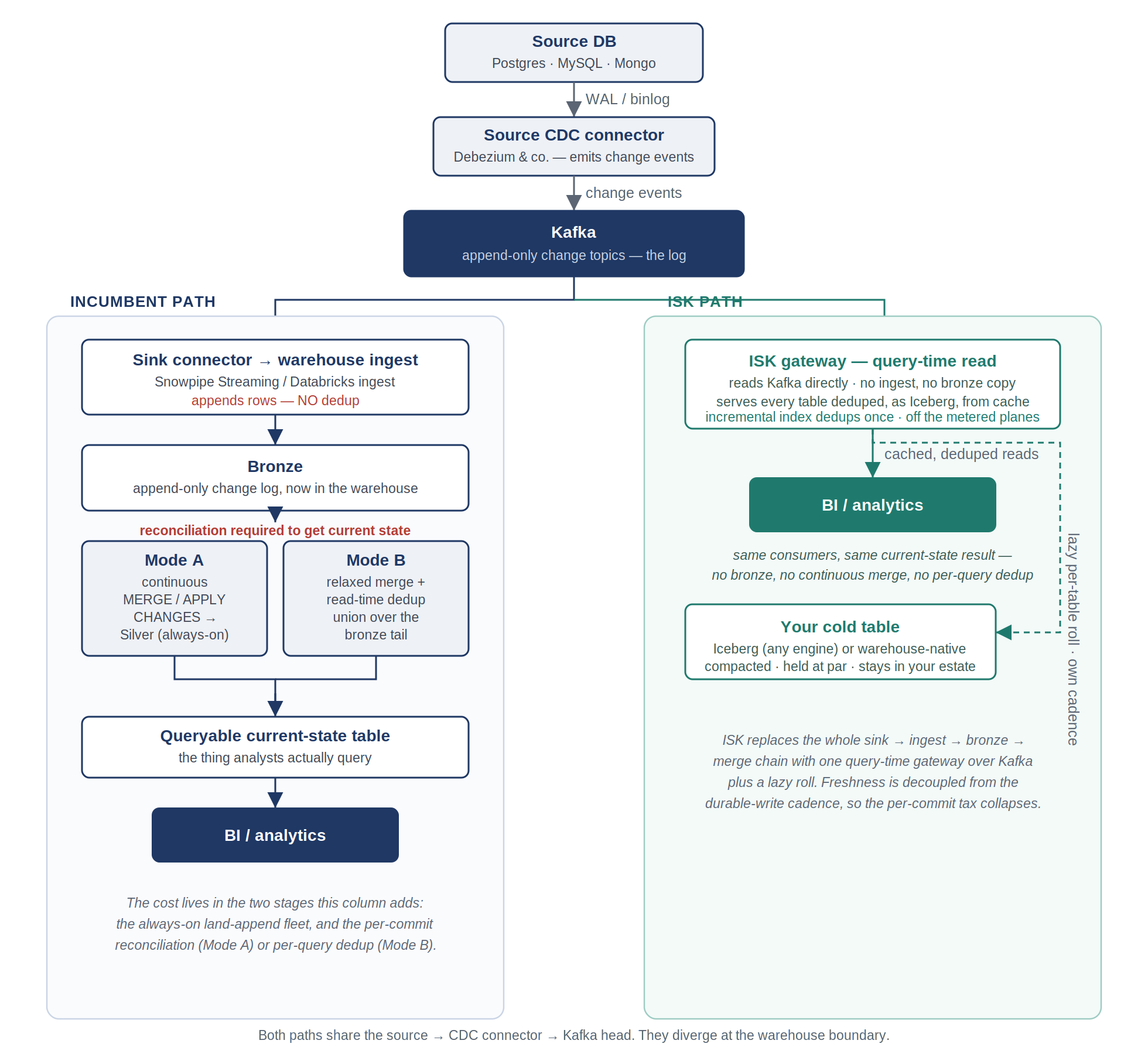
The shared head - source to Kafka

A source CDC connector (Debezium and the like) tails the source database’s write-ahead log or binlog and emits a stream of change events - insert, update, delete, keyed by primary key. Those events land in Kafka as append-only change topics - a durable, ordered log of what changed, not a current-state table. This head is identical on every path, ISK included, which is why the model counts only what happens after the Kafka boundary. The paths diverge at the warehouse edge.

The incumbent path - the landing is append-only, so reconciliation is mandatory

To get Kafka into the warehouse, a sink connector (or Snowflake’s Snowpipe Streaming, or the equivalent Databricks streaming ingest) writes the change events into a table. The key fact is that this landing is append-only. Snowpipe Streaming appends rows; the Databricks ingest path appends rows; neither deduplicates by key. What you have on the other side is a bronze table that is a second copy of the change log - the same stream of inserts, updates and deletes - not the current-state table anyone wants to query. (This is true whether bronze is a standard or a managed-Iceberg table; the ingest is append-only either way.)

Turning that append-only bronze into a current-state table you can join against is the reconciliation step - and it is where Mode A and Mode B live. Mode A runs a continuous MERGE / APPLY CHANGES that collapses the log into a silver current-state table on the freshness clock. Mode B leaves bronze relaxed and does the dedup at read time, as a union with a window function over the un-merged tail. Same requirement on both platforms; only the syntax differs. This is the unavoidable part: because the warehouse only ever ingests append-only, you must pay one of these two to get current state, and that payment is the per-commit tax the rest of this post is about.

The ISK path - collapse the chain

ISK isn’t another pipeline - it’s a query-time gateway. It reads the Kafka log directly, at query time, and never ingests - so the entire sink → ingest → bronze chain is eliminated, not relocated. There is no second append-only copy in the warehouse, and everything in Kafka is queryable the instant it’s produced, with no ingest lag. An incrementally-maintained key→offset index does the dedup once (so the read is not Mode B’s per-query scan over raw rows), a Parquet cache serves repeats, and materialization is lazy - nothing is consumed until a query asks for it. Each table then rolls to the customer’s own compacted cold table - Iceberg or warehouse-native - lazily, at its own volume-appropriate cadence. Freshness is decoupled from the durable-write cadence, which is the single move that collapses the per-commit tax. The cold table is held at par in the model on purpose: it lives in the same estate either way.

The three read paths - and why two of them only look alike

The tell is the read path. Mode A keeps a current-state table continuously, so reads are plain - the cost is the always-on merge on the write side. Mode B and ISK both close the freshness gap with a read-time union over a hot tail, which is exactly why they get conflated - but they are not the same union. Mode B unions the raw, un-merged bronze tail and has to dedup it on every query; ISK unions a hot window the head has already deduped, so the read is a cheap overlay and the dedup was paid once, upstream. Same shape, opposite cost behaviour - which is the whole reason ISK isn’t just a lambda.

‍